In my last post, we embarked on a journey to explore the various Machine Learning algorithms in detail. Starting with one of the most basic algorithms, we saw two types of regressions, namely Linear and Polynomial Regression. If you missed my post or would want to brush through the concepts, you can find it here: Linear and Polynomial Regression.
In this post, we will explore three concepts, Underfitting, Overfitting, and Regularization. The relation between regularization and overfitting is that regularization reduces the overfitting of the machine learning model. If this sounds Latin to you, don’t worry, continue ahead and things will start making sense. Let’s get to it.
Table of contents
- Underfitting
- Overfitting
- Optimal Fit
- Loss Function
- Regularization
- Ridge Regression / L2 Regularization
- Lasso Regression / L1 Regularization
- Elastic Net Regression
Underfitting
Generally, when a machine learning model is said to be “underfitting” it means that our model fails to produce good results because of an oversimplified model. Such a model can neither model the training data nor generalize over new data. When such a situation occurs, we say that the model has “high bias”.
“Bias is the difference between the average prediction of our model and the correct value which we are trying to predict. A model with high bias pays very little attention to the training data and oversimplifies the model. It always leads to a high error on training and test data.”
Hence, an underfit model performs poorly on training as well as testing data.
Overfitting
It is the opposite case of underfitting. Here, our model produces good results on training data but performs poorly on testing data. This happens because our model fits the training data so well that it leaves very little or no room for generalization over new data. When overfitting occurs, we say that the model has “high variance”.
“Variance is the amount that the estimate of the target function will change if different training data was used.”
Overfitting can be best explained as:

Optimal Fit
Needless to say, an optimally fit model is the one that performs well on training as well as testing data with room for generalizing over new data observations.
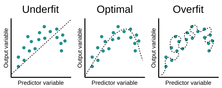
In the case of regression problems, these 3 concepts can be explained as:
We can solve the problem of underfitting by increasing the training data used. Another method is to increase the number of features (derive new features from existing ones or consider more parameters in training the model).
Some of the approaches to solving the problem of overfitting are:
- Cross-Validation
- Train with more data
- Remove features
- Early stopping
- Regularization
- Ensembling
Among these, we will be looking at Regularization in this post.
Regularization
The word “regularize” means to make things regular or acceptable. This is exactly why we use it for. Regularization is a form of regression used to reduce the error by fitting a function appropriately on the given training set and avoid overfitting. It discourages the fitting of a complex model, thus reducing the variance and chances of overfitting. It is used in the case of multicollinearity (when independent variables are highly correlated).
Recall that in the last post, we discussed the equation of Linear Regression. Let \(\hat{y}\) be the prediction made.
\[y = w_1x_1 +w_2x_2 + w_3x_3 + ... + w_nx_n + b\]We also introduced the concept of loss functions. We will use one such loss function in this post - Residual Sum of Squares (RSS). It can be mathematically given as:
\[L = RSS = \sum_{i=1}^{m} (y_i - \hat{y_i})^2\]Regularization can be of two kinds, Ridge and Lasso Regression. Using the above equations as a base, we will discuss each one in detail.
Ridge Regression / L2 Regularization
In this regression, we add a penalty term to the RSS loss function. Our modified loss function now becomes:
\[L_2 = \sum^{m}_{i=1} (y_i - \hat{y_i})^2 + \lambda \sum^{n}_{j=1} {w_j}^2 = RSS + \lambda \sum^{n}_{j=1} {w_j}^2\]Here, \(\lambda\) is called the “tuning parameter” which decides how heavily we want to penalize the flexibility of our model. If we look closely, we might observe that if \(\lambda=0\), it performs like linear regression and as \(\lambda \rightarrow \inf\), the impact of the shrinkage penalty grows, and the ridge regression coefficient estimates will approach zero. As can be seen, selecting a good value of \(\lambda\) is critical. The coefficient estimates produced by this method are sometimes also known as the “L2 norm”.
Lasso Regression / L1 Regularization
| This regression adopts the same idea as Ridge Regression with a change in the penalty term. Instead of \({w_j}^2\), we use $$ | w_j | $$. Thus our new loss function becomes: |
In statistics, this is sometimes called the “L1 norm”.
Note: The tuning parameter \(\lambda\) controls the impact on bias and variance. As the value of \(\lambda\) rises, it reduces the value of coefficients and thus reducing the variance. Till a point, this increase in \(\lambda\) is beneficial as it is only reducing the variance (hence avoiding overfitting), without losing any important properties in the data. But after a certain value, the model starts losing important properties, giving rise to bias in the model and thus underfitting. Therefore, the value of \(\lambda\) should be carefully selected.
Elastic Net Regression
This is a hybrid kind of regression that brings the best of both the worlds (Ridge and Lasso Regressions). This is done by including penalty terms by both methods. The loss function for Elastic Net regression can be given by:
\[L_{ElasticNet} = \sum^{m}_{i=1} (y_i - \hat{y_i})^2 + {\lambda}_1 \sum^{n}_{j=1} {w_j}^2 + {\lambda}_2 \sum^{n}_{j=1} |w_j| = RSS + {\lambda}_1 \sum^{n}_{j=1} {w_j}^2 + {\lambda}_2 \sum^{n}_{j=1} |w_j|\]This regression is generally found to outperform Ridge and Lasso Regression.
Regularizations are truly an integral part of any machine learning project. It helps our model make realistic predictions.
Arigato!
Got any questions or suggestions? Want to share any thoughts or ideas with me? Feel free to reach out to me on LinkedIn. Always happy to help!
Also, you can view by other works on GitHub and my blog.
Till then, see you in my next post!