Diving Deep into Linear Regression and Polynomial Regression

In my previous post, we explored different branches of AI. I’m almost certain that now you might want to learn about these branches in greater detail. Worry not, I’ll surely open the gates to these subsets in the posts to come. If you missed my post, you can find it at the following link: Branches of Artificial Intelligence.

Previously, we discussed Machine Learning. We also discussed its subsets - Supervised Learning, Unsupervised Learning, and Reinforcement Learning. In this post, we’ll be discussing one of the most fundamental algorithms in Supervised Learning - Regressions. Regressions can be of many types. You might have come across some types of regressions previously or maybe are hearing about it for the first time. Particularly, we’ll be looking at two types of regression in this article, namely, “Linear Regression” and “Polynomial Regression” along with their mathematical formulae and python code.

Before getting into these types, let’s first understand what is “Regression”.

“Regression is a statistical approach of the strength of the relationship of a dependent variable with a set of independent variables.”

Confused? Let’s understand it with an analogy. Imagine that you want to buy a house. Now I think you will agree with me that the price of the house will be based on the size of the house (in sq. feet) and its location (there can be many more parameters on which the price of the house can be dependent, but for simplicity, let’s assume these two to be the primary drivers.) If you opt for a larger house, naturally the cost of the house will shoot up and if your dream home is a penthouse apartment in Manhattan with a skyline view, it’s going to be way costlier that one in Queens (well, my personal choice would be home in Monaco!)

Here, the size and location of the house will be the independent variables. As the name suggests, changing one has no effect on the other, meaning they are “independent” of one another. The price of the house will be the dependent variable, as it depends on the size and location. Thus, “Regression Analysis” is the method of predicting the dependent variable by making use of the independent variable(s).

Without further due, let’s dive into Linear and Polynomial Regression.

Table of contents

1. Linear Regression
2. Polynomial Regression
3. Initializing Equation Coefficients
4. Loss Function
5. Stochastic Gradient Descent (SGD)
6. Python Code - Housing Price Dataset

Linear Regression

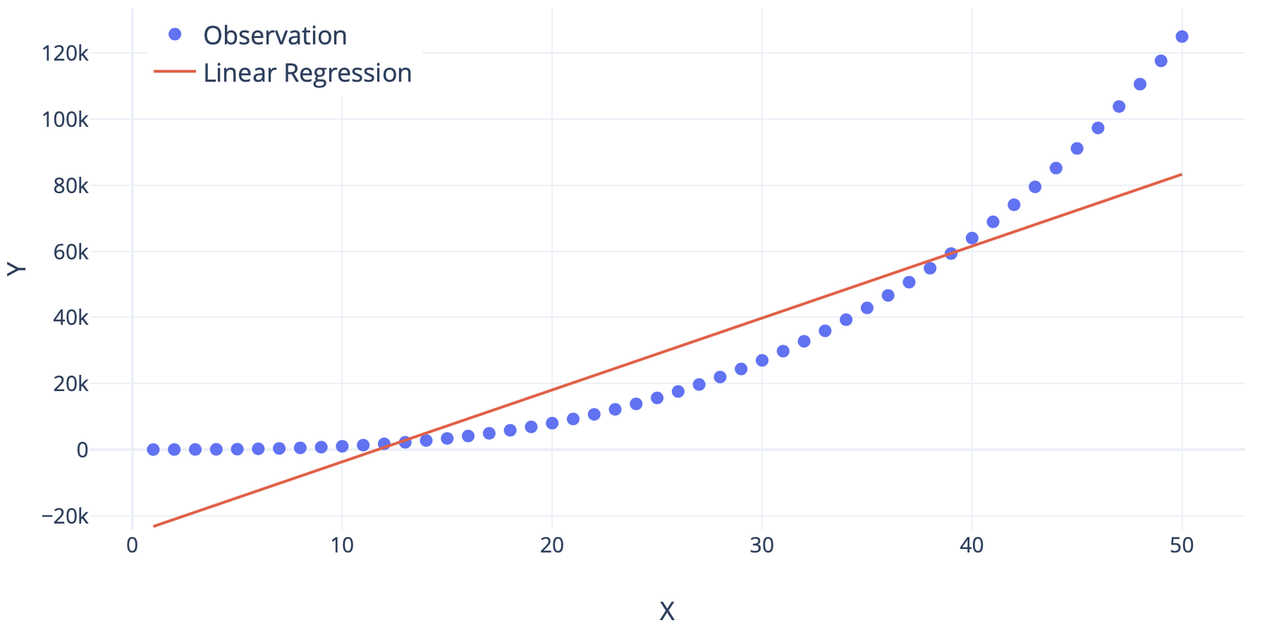
Linear Regression is a method of regression analysis that assumes a linear relationship between the dependent variables and the independent variables. This means that when we plot a graph between the dependent and independent variables, a straight line is formed. This is an approach to tackle problems that demand to make predictions as continuous values. Being the most basic algorithm, for any tasks where we wish to predict a continuous value, this is the first algorithm that is generally implemented.

In the case of only one independent variable, we call it “Simple Linear Regression.” As simple as that! Say, y is the dependent variable, x be the independent variable. Let w be the weight of the variable and b be the bias (bias can sometimes be zero). Weights and Bias are nothing but values that transform the independent variable into the dependent variable. Hence, mathematically,

If you find it difficult to understand, think of our analogy. The price of the house is in proportion to the size of the house. So our equation becomes:

In the case of many independent variables and the dependent variables, we call it “Multiple Linear Regression.” So, let X be a set of n independent features and W be the set of new weights for each value in X.

Our equation for multiple linear regression will be:

And correspondingly, we can also modify the equation for that of our analogy.

If predictions by this algorithm are agreeable to us, then we are happy to go! Simple, easy, and interpretable. But generally we observe that for real-world problems, this is not the case. In most of the real-world problems, the relationship between the dependent and the independent variables will not be linear, and in such a case, it is often found that linear regression performs poorly.

Polynomial Regression

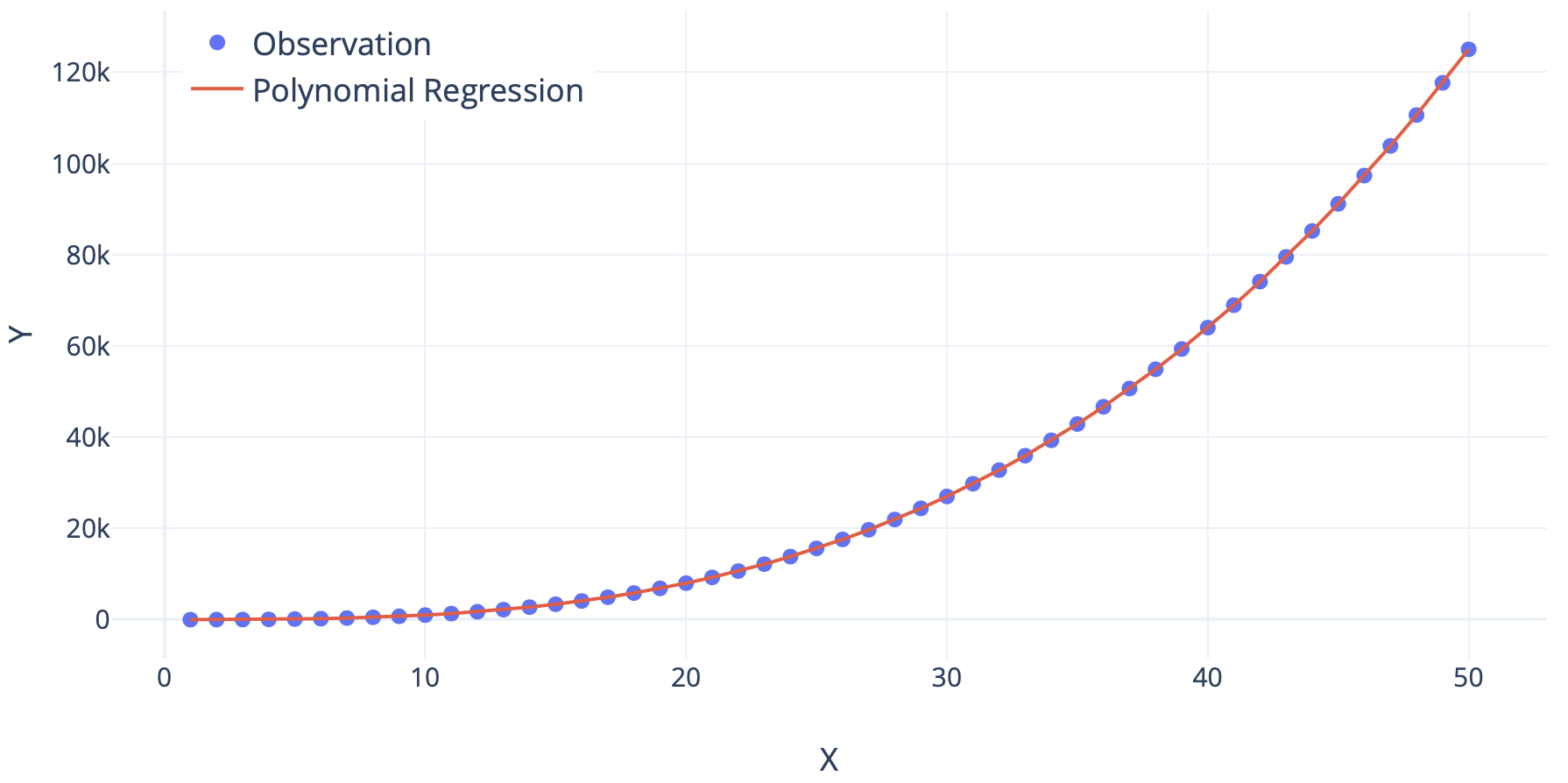
To tackle the problem of non-linearity, we introduce a slight tweak in our approach - Polynomial Regression. This method of regression analysis, the independent variables can be linearly or non-linearly dependent on the dependent variable. This helps us build complex curves that can contribute to devising more appropriate representations of the real-world scenarios.

Even polynomial regression can be classified as simple and multiple polynomial regression. The equation for simple polynomial regression can be given as:

Notice that the square of the independent variable has been considered. This introduces non-linearity.

On similar lines, the equation for multiple polynomial regression can be given as:

Where n, p, q, r can be integers that introduce non-linearity.

This approach has shown to outperform the linear regression techniques generally by showing the ability to take more complex relationships under the hood. But it’s important for this approach that we know how the values in X and variable y are related. It becomes more of a trial and error if this is not known. Also, this is prone to overfitting if powers are not carefully chosen.

Initializing Equation Coefficients

It might have crossed your mind, what values to assign to the coefficients w and b before the training process and how do these values get optimized during training? If we observe carefully, we will realize that it is these coefficients that we want to estimate during our training process, in order to make our ML model better at predictions.

The process of assigning the initial values is called ‘Initialization’. There are multiple ways to initialize the coefficients. Some of the common initializations are:

1. Zeros
2. Ones
3. Normal Distribution
4. Truncated Normal Distribution

To understand how to optimize these coefficients during training, we need to study about two concepts: “Loss Function” and “Stochastic Gradient Descent (SGD)”. These terms might sound a bit overwhelming, but don’t worry, I’ve got your back!

Loss Function

Let’s consider a multiple linear regression with two independent variables. Our equation will be:

In this equation, y is the true values and wi and b are the optimal coefficients. As we initialize with suboptimal coefficients, our results will also deviate from the optimal results. Thus, our equation, till the time we achieve optimal coefficients and thus optimal results, will be:

Here, the new \(\hat{y}\), \(\hat{w_i}\), and \(\hat{b}\) are the suboptimal values. From now on, we will refer \(y\) as the “True Value” and \(\hat{y}\) as the “Predicted Value”.

In mathematical optimization and decision theory, a Loss Function can be defined as a quantitative representation of how costly the prediction proves to be. More the deviation in the true and predicted values, greater is the cost, and worse is the prediction made.

There are several ways to define a loss function based on the type of task at hand (regression or classification). Some of the loss functions for regression are:

1. Squared Error Loss
2. Mean Squared Logarithmic Error Loss
3. Mean Absolute Error Loss

We’ll look into them in detail in the posts to come.

Stochastic Gradient Descent (SGD)

We need to optimize \(w_i\) and \(b\) towards the optimal coefficients and thus obtain results as close to the actual values. In order to do so, we use optimizers. These optimizers employ the use of mathematical functions to move the coefficient values closer to the optimal values as it trains. There are a number of optimizers that we can use. But, let’s look at one to understand how an optimizer works. The one we will be focusing on is Stochastic Gradient Descent (SGD).

Let \(L\) be a loss function (could be any one of the 3 mentioned above or even other than these). The mathematical equation for this is:

Where \(η\) is the step size (also called learning rate) and it is multiplied with the partial derivative of the loss function with respect to the coefficient that is being updated.

The beauty of this equation is that without any human intervention, as training proceeds, it will optimize the coefficients. It does so by minimizing the loss function. Thus, this process is also called “Minimizing the Loss Function”.

To get a clear understanding of how this works, let’s say there are multiple hills and you are standing on the crest of one of them. If I were to tell you to reach the bottom-most point and you must take a step one at a time. Though there is one condition. At any given time, your next step must be in the direction of the steepest descent at that point. The way you would come down the hill is how gradient descent works!

There can be certain downsides to SGD. Also, there are many different optimizers that work in different ways. We shall discuss them in the future.

Goal Achieved, Linear, and Polynomial Regression learned!

So till now, we learned about Linear and Polynomial Regression.

Now let’s look at the code to apply Linear and Polynomial Regression on the ‘Housing Price Dataset’.

Python Code - Housing Price Dataset

The dataset used for this tutorial is House Price Prediction. It has been modified by me to make it simpler to understand. The entire code (Jupyter Notebook) and the dataset can be found at: Linear and Polynomial Regression Jupyter Notebook

The modified dataset “data.csv” contains 3 independent variables and 1 dependent variable.

Independent Variables:

1stFlrSF - First Floor square feet 2ndFlrSF - Second floor square feet YearBuilt - Original construction date

Dependent Variables:

SalePrice - the property’s sale price in dollars. (This is the target variable that you’re trying to predict.)

If you wish to work on the complete dataset, it can be found at: House Prices - Advanced Regression Techniques

Let’s get into the code right away!

Step 1. Importing Python Libraries

A short description of all the libraries:

datetime - supplies classes for manipulating dates and times.

sys - provides access to some variables used or maintained by the interpreter and to functions that interact strongly with the interpreter

pandas - a fast, powerful, flexible, and easy to use open-source data analysis and manipulation tool, built on top of the Python programming language.

scikit-learn - contains a lot of efficient tools for machine learning and statistical modeling including classification, regression, clustering and dimensionality reduction (imported as sklearn)

math - provides access to the mathematical functions defined by the C standard

1
2
3
4
5
6
7
8
import datetime as dt
import sys
import pandas as pd
from sklearn.model_selection import train_test_split
from sklearn.linear_model import LinearRegression
from sklearn.metrics import mean_squared_error
from sklearn.preprocessing import PolynomialFeatures 
from math import sqrt

Step 2. Reading the Dataset as a Dataframe using Pandas

The file “data.csv” needs to be called first for using it to train our model. We read it as a pandas dataframe and assign it to variable df. For this, we will make use of the read_csv() function.

1
df = pd.read_csv("data.csv")

Step 3. Initializing the Independent and the Dependent Variables

We now need to separate the dependent variable (y) from the independent variable(s) (X). It can be done by running the following code:

1
2
X = df.drop("SalePrice", 1)
y = df["SalePrice"]

Step 4. Training and Testing Data

Two sets of data are needed for our task, one for training and the other for testing. Sklearn provides a function train_test_split() to do so. For the task that we intend to perform, we’ll be using 80% of the total data for training and the remaining 20% for testing.

X_train - part of X used for training y_train - part of y used for training X_test - part of X used for testing y_test - part of y used for testing

1
X_train, X_test, y_train, y_test = train_test_split(X, y, test_size=0.20, random_state=42)

Step 5. Linear Regression Model

At last, our Linear Regression model is finally here! The variable “model” creates an instance of our Linear Regression model. In the second line, we can see “fit” function. What fit() function really does is that it trains our model using the training data. Now our model has been trained. We will use the predict() function to obtain predictions on X_test. These predictions can be compared with actual values to determine how our model has performed.

1
2
3
model_lin = LinearRegression()
model_lin.fit(X_train, y_train)
y_pred_lin = model_lin.predict(X_test)

Step 6. Polynomial Features

In order to obtain polynomially related features, scikit-learn offers a function named PolynomialFeatures(). If a variable p is related to q in quadratic terms, then p² is linearly dependent on q. Thus, we will generate features of higher power and feed them to a linear regression model. This will enable us to implement polynomial regression. In the following code, X_poly will act as the new X_train which will be used for the training task.

1
2
3
poly = PolynomialFeatures(degree = 4) 
X_poly = poly.fit_transform(X_train)
poly.fit(X_poly, y_train)

Step 7. Polynomial Regression Model

Similar to Linear Regression, we use Linear Regression model with polynomial features as input.

1
2
3
model_poly = LinearRegression() 
model_poly.fit(X_poly, y_train)
y_pred_poly = model_poly.predict(poly.fit_transform(X_test))

Step 8. Tabulating Results

This step is to create a new dataframe that stores the actual/true as well as predicted values by both models. This is done using the function DataFrame().

1
2
3
4
5
results = pd.DataFrame({
    "LinPred": y_pred_lin,
    "PolyPred": y_pred_poly,
    "TrueValues": y_test
})

Step 9. Evaluation Metrics - Root Mean Square Error (RMSE)

How do we quantitatively evaluate how our model has performed? For this purpose, we use something called “Evaluation Metrics” which compares the predicted and actual values and gives us a number. Depending on how high or low the value is, we can say how good our model is. One such evaluation metric is the “Root Mean Square Error” or simply RMSE. I’m sure you might have studied about it sometime. In case you wish to know more about RMSE, check out this article: What does RMSE really mean?

1
2
3
4
5
rmse_lin = sqrt(mean_squared_error(results["TrueValues"], results["LinPred"]))
rmse_poly = sqrt(mean_squared_error(results["TrueValues"], results["PolyPred"]))

print("RMSE (Linear Regression): ", rmse_lin)
print("RMSE (Polynomial Regression): ", rmse_poly)

RMSE obtained by Linear Regression is 46321.133955685014 and that by Polynomial Regression is 36741.49042680656.

I know the RMSEs are too bad. We will use the complete data, perform better feature engineering, and implement more robust algorithms to obtain better results in the future.

We can observe one thing that RMSE for the Polynomial Regression is better than that for the Linear Regression. Hence, we can conclude that Polynomial Regression generally outperforms Linear Regression as Polynomial basically fits a wide range of curvature.

Thank you for reading!

Got any questions or suggestions? Want to share any thoughts or ideas with me? Feel free to reach out to me on LinkedIn. Always happy to help!

Also, you can view by other works on GitHub and my blog.

Till then, see you in my next post!